Polynomiography Applet Instructions

Introduction
The Three Main Windows
The Coefficients Table
The Settings Window
The Graph Window
Summary

Introduction to the Polynomiography Java Applet

It is useful for the user of this software to keep in mind the following points:

This software allows you to create images of polynomial equations such as 2x^ 4- 7x^ 3+ 3x^ 2-5x+ 1, i. e. (2 times x to the power of 4, minus 7 times x to the power of 3, plus 3 times x to the power 2, minus 5 times x, plus 1). Here, the degree of the polynomial is 4. The polynomial coefficients are 2, -7, 3, -5, and 1. It may happen that a coefficient is zero. However, the user will only enter the equation as numbers using its coefficients. Thus, no knowledge of polynomials is needed to use the software.
An overview of polynomiography is this: a polynomial has "roots," as many as its degree. The roots can be imagined as points in the Euclidean plane. They divide all the other points among themselves based on some rules. These rules are dictated by the use of some functions called "iteration functions."
The relationship between polynomiography, a polynomiographer, and the underlying polynomial is somewhat analogous to the relationship between photography, a photographer, and the photographic model. Thus, the user would first need to enter a polynomial, and then select particular parameter( s) before generating an image.
The Java Applet is several times slower than the PC version. Hence, only a small canvas is allowed.

The Three Main Windows

When the applet appears, you will see the following:

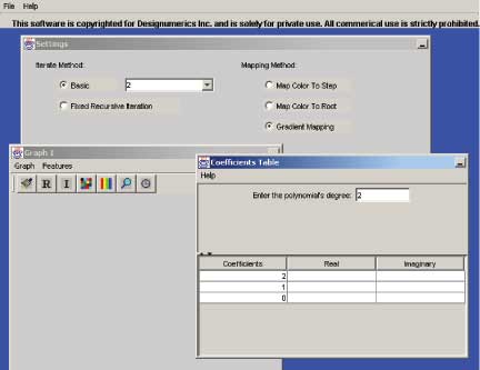
The three windows as they appear when Java applet loads

As you can see, there are 3 main windows: The Coefficients Table, the Settings window, and the Graph window. We'll consider each one individually, but by doing so, it will be clear how to use them together to easily generate images.

The Coefficients Table

The Coefficients Table:

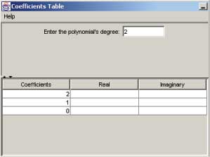
The table consists of a text field at the top of the table and a grid at the bottom. The field at the top asks for the degree of the polynomial. In other words, it wants to know what the greatest exponent of the polynomial is. You are allowed to have polynomials with degrees from 1 to 12. Right now, the degree is 2, so the polynomial is of the form ax^ 2 + bx + c. Let's say we want a polynomial of degree of 4. We can just type 4 into the field and immediately press Enter. If you forget to press Enter, the table will not change size. So, you must click back inside the text field, and then press Enter. Once we do that, the table expands to 5 rows, labeled from 4 to 0.

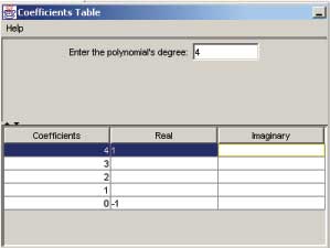
Say we want to enter a polynomial, perhaps x^ 4 – 1. So, the coefficient for x^ 4 is 1. As a complex number, 1 is 1 + 0i so its real part is 1 and its imaginary part is 0. To enter the coefficient for the 4 th power, go to the row labeled 4. Then type 1 in the "Real" field. -1 is the constant term in the polynomial. -1 is -1 + 0i as a complex number. In the table, constants go into the row labeled 0. So, in that row, enter -1 in the "Real" field. If the polynomial was x^ 4 + (5 + 2i) x – 1, you would need to enter another term. To enter the (5 + 2i) x term, notice the (5 + 2i) is the coefficient of x to the 1 st power. So, you would go to the row labeled 1, and enter 5 in the "Real" field and 2 in the "Imaginary" field.

Note that zero coefficients do not need to be entered into the table.

After entering all the coefficients for the polynomial you want to draw, you must hit Enter.

The Settings Windows

The Settings window:

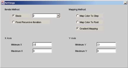
This window controls the main features of the image you're going to draw.

In the upper left region, you have the option of choosing either Basic or Fixed Recursive Iteration as the Iteration Method. Without dwelling on the meaning behind these terms, we'll consider either option. If you choose the Basic combo box, then you should enter any number between 2 and 32 inclusive. Entering different numbers produces different images of the same polynomial. This is analogous to taking pictures of the same object using different camera lenses. Changing the lens will produce a different picture of the same object. The default value for Basic is 2, which is equivalent to using Newton's method. Your other choice is to select Fixed Recursive Iteration, by clicking on its radio button. This method will produce different images than those obtained when using the Basic method.

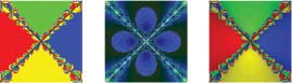
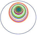
In the upper right region of the Settings window, you can select a mapping method. Map Color To Root maps a color to every pixel that converges to the same root. So, in the first image above, all the green pixels converge to the same root. The same goes for the red, yellow, and blue pixels. Map Color To Step maps a color to all pixels that are the same number of iterations away from their respective roots. So, in the second image above, all the pixels of the same blue shade are all the same number of iterations away from their roots. Gradient Mapping is a combination of the previous two mapping techniques. Every pixel first has its color mapped to a root, like Map Color To Root. But then the color is darkened, depending on how far away it is from the root. Thus, Map Color To Step is also occurring. For example, in the last image above, all the green pixels converge to the same root, but the darker green pixels require more iterations to converge then the lighter green pixels.

In the lower left and right, you can control the axes of the image. You're allowed to manipulate the minimum and maximum values of the x and y axes by changing the values in the appropriate fields.

The Graph Window

The Graph window:

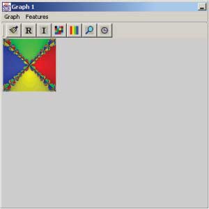
The Graph Window is where images are drawn and visually manipulated. Once a polynomial has been entered in the Coefficients Table and its settings have been configured, you're ready to generate an image. To do so, click on the paint brush icon in the toolbar of the Graph Window. You'll see a progress bar pop up briefly as the image is generated. To display a list of roots for the polynomial, click on the "R" icon in the toolbar. A dialog box will appear with the list of roots.

Let's say you want to see the coordinates of an iteration path starting at a particular coordinate. To do this, first click on the coordinate in the image that you want to see a path for. Once you click, you'll see a white dot where you clicked. Then, click on the "I" icon in the toolbar. A dialog box will appear, showing the path from the first coordinate in the path to the root.

The next two icons in the toolbar deal with manipulating the colors of the image. The first button allows you to replace one color in the image with another. So, click on a color in the image you want to change. Once you click, you will see a white dot where you clicked. Then click on the button. A large dialog box will appear, allowing you to select practically any color you want. Choose any color you like and press OK. Now, the color you selected has been replaced throughout the image with the new color. The second button also changes color, but changes the color of an entire gradient. The procedure for color changing is the same as for the first button, but the entire gradient experiences the color change.

The next button is the magnifying glass, representing the zoom feature. To zoom in on an area, click on the spot in the image that you want to be the center of the zoomed in image. Then click on the magnifying glass. A progress bar will pop up briefly, and then the zoomed in image will appear.

The last button, when clicked, displays the amount of time it took to display the last generated image.

Also notice that the functions of these buttons can be performed by selecting the appropriate menu items in the Graph and Features menus in the Graph window. While on the subject of the menus, there are two features that do not have a toolbar button, but are available in the Features menu. One of these features is entitled 'Clean Up Image' and simply removes the white pixel, if present, that appears when clicking on an image. The other feature involves two menu items, 'Enlarge Image' and 'Shrink Image. ' 'Enlarge Image' allows an image of normal size to be enlarged. 'Shrink Image' returns enlarged images to their original size.

Multiple Graph Windows:
It is possible to have multiple GraphWindows open, which is useful to display multiple images. To add a GraphWindow, go to the File menu and select New Graph Window.

Summary

Image generation is very simple in this applet and follows a simple pattern. First, enter the polynomial in the Coefficients Table. Then go to the Settings window and change any settings you like. Finally, go to the Graph Window and generate the image, and do any image manipulation you desire.

fetishroom.net